I know I can do this in Excel - just forotten HOW!

So,

I have a speadsheet set up to look at my energy costs.

A calculation is done and the cell produces a positive value if it is cheaper today and a negative value if it is more expensive today (it is looking at the tracker rate for energy conpared to the standard tariff. If the tracker is cheaper, it would save money and produce a positive value).

So, looking at conditional formatting applied to the cell.

I can apply conditional formatting to get the cell value to turn the value green (if positve and saving money) or red if negative - but not both together - ie same cell will have green text or red depending on whether value is positive or negative.

I know I can do this and have done so in the past but cannot figure out how this morning!



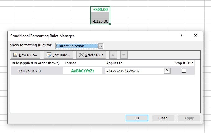
Above is an example (and yes, I know there is only one rule showing). Here three cells AW236, AW236 & AW237 have the same formatting applied, cell AW236 has a positive value (and has gone green as wanted), cell AW237 hasn't gone green as wanted. I know I need a second rule applied to these cells such that if <0, the cells will be red.

However, there seems to be no option or way to get a second rule that says 'Cell Value <0', the second rule seems to have to be a formula applied to the same cells - and this is where I am coming unstuck.

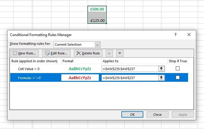
I have tried the following - but as you can see, the formula (my fault undoubetdly) isn't working.



How do I apply the second rule to the cells to get the desired result - negative values in red?

Thanks folks!

Art

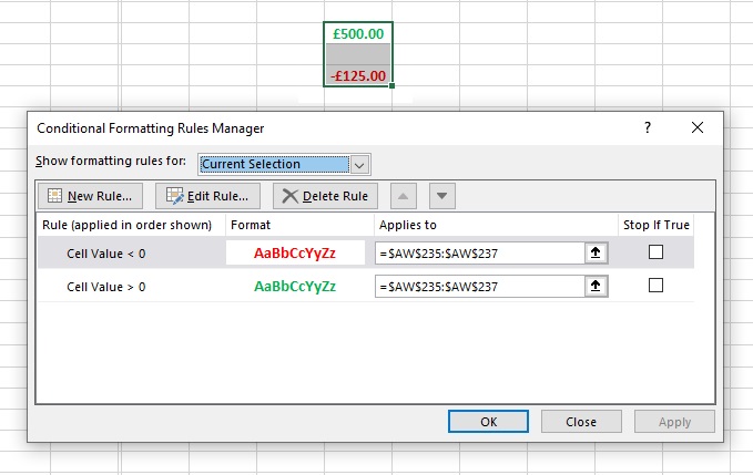
UPDATE: A sudden flash of inspiration. Just create a new rule the same way as the first:



And it does what I wanted it to do! *forehead slap*

Art