Help needed with Excel Attendance Sheet

ReallyFrustratd said:

id like to make the MONTH cell a drop down list

You use the Data tab, Data validation facility to do this.

If you want a coherent explanation then look in Excel Help. Here's the relevant extract from Excel 2007 Help. Excel 2007 Help - Data Validation.pdf

My example:
- I have written them in what seems to me to be the order of easiest explanation.
- You'd actually set them up in the reverse order - step 3, step 2, step 1.

1 The result - my dropdown list. I select the cell then click on the dropdown arrow that appears next to it.


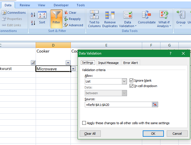
2 To set this up, select the whole column [or individual cells] where you want the dropdown to appear then click on the Data tab then the Data validation control. You need to
- select In-cell dropdown
- set the Allow entry to List
- in Source, enter the worksheet name & cell range where you have written the allowable entries - you will generally want to use absolute cell references such as those shown [$ in a cell address means absolute and will not vary as you copy the formula all the way down your column - look this up if you are not familiar with it because it needs a bit of getting used to].


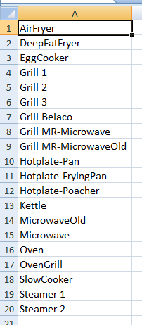
3 Write out the list of allowable entries that will appear in your dropdown list.


Job done.

Denis

As for hiding cells depending on the month selected I think that might well be handled as a Conditional formatting matter - a topic about which you are an expert
- Blanking out the cell content [so you do not see it] rather than hiding the cells can be easier to set up and easier to deal with.
- I suspect that the easiest way to do it would be to put a second column next to your existing list of months [in your Config worksheet] containing the number of days in each month.
- You can then refer to the list using a XLookup function, assuming Office 365, [which used to be VLookup & HLookup in earlier versions] in your row 16 cells and base a Conditional format on the results.

- It's possible that you might find it easiest to add a row somewhere with the nitty gritty of the calculation so that row 16 can just apply formats that refer to the calculation's results.

- You might find something in your Date-Time functions to help you decide how to adjust February for Leap years.

- If not, see Method to determine whether a year is a leap year - MSDocs.
- The reason I think Excel 365 might have a function to help with this is that the MSDocs page 'Applies to' list stops at Excel 2016 so there is something different about Excel 2019 & Excel 365. But I could not find anything useful in Excel functions (alphabetical) - OfficeSupport]

Denis