Conditional formating

Page 2 of 3 FirstFirst 123 LastLast

  1. Posts : 119
    Windows 11 Home 64 Bit
       #11

    Hi again,

    After a little thought you could use this in a cell to combine both checks for the conditional formula.

    Inserted into cell B7,
    =IF(B2="W","",IF(B2="L",IF(B3<8,2,"")))

    Inserted into cell B8,
    =IF(B4="W","",IF(B4="L",IF(B5<8,2,"")))

    This is looking at both cells (B2 & B3) & (B4 & B5) for the comparison checks. Change cell references (B2 & B3) & (B4 & B5) for each cell you want to check.

    Conditional formating-excel-conditional-formating.jpg

    The conditional formula for cell B2 is =B7=2, for the range of your cells.
    Conditional formating-condition1-formating.jpg

    The conditional formula for cell B4 is =B8=2, for the range of your cells.
    Conditional formating-condition2-formating.jpg
      My Computer


  2. Posts : 119
    Windows 11 Home 64 Bit
       #12

    Lottiemansion said:
    Inserted into cell B7,
    =IF(B2="W","",IF(B2="L",IF(B3<8,2,"")))
    Inserted into cell B8,
    =IF(B4="W","",IF(B4="L",IF(B5<8,2,"")))
    If you need the Highlight for cell value above "8", then the formulas should be: -

    Inserted into cell B7,
    =IF(B2="W","",IF(B2="L",IF(B3>8,2,"")))

    Inserted into cell B8,
    =IF(B4="W","",IF(B4="L",IF(B5>8,2,"")))

    I hope it helps you...
      My Computer


  3. Posts : 174
    microsoft windows 10
    Thread Starter
       #13

    I have just tried the advice and when I enter into a cell =if(A4<8,1,0) it works ok but sometimes the cells I am checking are blank and it will put a 1 in the result, how can I resolve this please.
    Len
      My Computer


  4. Posts : 119
    Windows 11 Home 64 Bit
       #14

    donnylad said:
    I have just tried the advice and when I enter into a cell =if(A4<8,1,0) it works ok but sometimes the cells I am checking are blank and it will put a 1 in the result, how can I resolve this please.
    Len
    If you change the cell to this: -

    =if(A4="","",if(A4<8,1,0))

    It should keep the cell blank.
      My Computer


  5. Posts : 1,524
    Win10 Pro
       #15

    Hi donnylad. I found a formula on the web that will do just what you want without adding any extra cells but it requires that your data be arranged in columns rather than rows. If you are willing to use the Transform function to do this I can adapt what I found to give you the results you are asking for. Let me know if you can live will columns in lieu of rows and I’ll post the formula later today.
    Bob
      My Computers


  6. Posts : 174
    microsoft windows 10
    Thread Starter
       #16

    Not sure ifI can Bob I am going to try what I have up to now but you can post it and I will see if it will do my needs.
    Thanks
    Len
      My Computer


  7. Posts : 174
    microsoft windows 10
    Thread Starter
       #17

    Hi Lottie, Thanks for your help its working fine.
    Len
      My Computer


  8. Posts : 1,524
    Win10 Pro
       #18

    donnylad said:
    Not sure ifI can Bob I am going to try what I have up to now but you can post it and I will see if it will do my needs.
    Thanks
    Len
    Here you go:
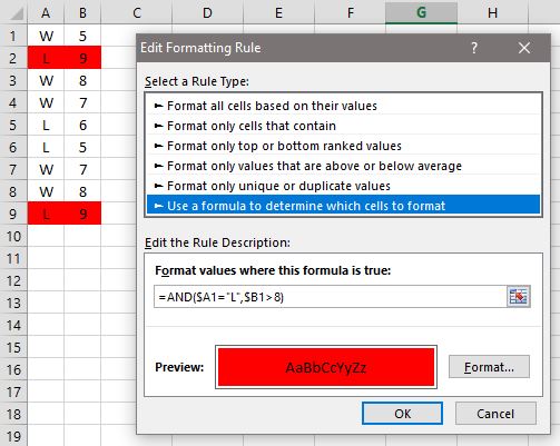
    Conditional formating-excelformat.jpg
    The reason that the data needs to be arranged into columns is that the relative addressing that is used with conditional formatting does not work when the comparisons are made across rows. Maybe someone else knows how to modify the formula but I haven't yet discovered how.

    BTW here's where I found the formula: Use Conditional Formatting with Multiple Conditions - YouTube
    In case the video won't play just search on "Youtube Use Conditional Formatting with Multiple Conditions"
    Bob
      My Computers


  9. Posts : 174
    microsoft windows 10
    Thread Starter
       #19

    Thanks Bob I am looking at it now and reply.
    Len
      My Computer


  10. Posts : 119
    Windows 11 Home 64 Bit
       #20

    Hi,

    If the conditional formula above (BOB's) is changed to this: -

    =AND(B2="L",B3<8) for row one, applying to your cells

    and

    =AND(B4="L",B5<8) for row two, applying to your cells.

    It does work across the spread sheet. However, the problem of highlighting an empty cell still exists as this equates to zero or a null.

    Therefore use this formula: -

    =IF(B3="","",AND(B2="L",B3<8)) for row one.

    and

    =IF(B5="","",AND(B4="L",B5<8)) for row two. Sorted I think?

    Attachment 221352
    Attached Thumbnails Attached Thumbnails Conditional formating-excel-conditional-formating-2.jpg  
      My Computer


  Related Discussions
Our Sites
Site Links
About Us
Windows 10 Forums is an independent web site and has not been authorized, sponsored, or otherwise approved by Microsoft Corporation. "Windows 10" and related materials are trademarks of Microsoft Corp.

© Designer Media Ltd
All times are GMT -5. The time now is 23:26.
Find Us


Windows 10 Forums